root

public

mirror of https://github.com/01-edu/public.git

eslopfer f8fae31cf0 docs(ai-audits): fix format errors, rephrase, and typos		2 years ago
..
audit	docs(ai-audits): fix format errors, rephrase, and typos	2 years ago
data	docs(classification): rename path to match ref	2 years ago
README.md	docs(classification): rename path to match ref	2 years ago
w2_day2_ex2_q1.png	docs(classification): rename path to match ref	2 years ago
w2_day2_ex3_q1.png	docs(classification): rename path to match ref	2 years ago
w2_day2_ex3_q3.png	docs(classification): rename path to match ref	2 years ago
w2_day2_ex3_q5.png	docs(classification): rename path to match ref	2 years ago
w2_day2_ex3_q6.png	docs(classification): rename path to match ref	2 years ago

README.md

Classification

The goal of this day is to understand practical classification with Scikit Learn.

Today we will learn a different approach in Machine Learning: the classification which is a large domain in the field of statistics and machine learning. Generally, it can be broken down in two areas:

Binary classification, where we wish to group an outcome into one of two groups.
Multi-class classification, where we wish to group an outcome into one of multiple (more than two) groups.

You may wonder why the approach is different from regression and why we don't use regression and define a threshold from where the class would 1 else 0 - in binary classification. The main reason is that the linear regression is sensitive to outliers, hence the treshold would vary depending on the outliers in the data. The article mentioned explains this reason with plots. To keep things simple, we can say that the output needed in classification is a probability to belong to one of the classes. So, by definition the value output by the classification model has to be between 0 and 1. The linear regression can't satisfy this constraint.

In mathematics, there are functions with nice properties that take as input a real (-inf, inf) and output a value between 0 and 1, the most popular of them is the sigmoid - which is the inverse function of the logit, hence the name logistic regression.

Let's take a small example to have a better understanding of the steps needed to perform a logistic regression on a binary data. Let's assume that we want to predict the gender given the people' size (height).

Logistic regression steps:

Fit a sigmoid on the training data
Compute sigmoid(size)=0.7 because the sigmoid returns values between 0 and 1
Return the class: 0.7 > 0.5 => class 1. Thus, the gender is male

For the linear regression exercises, the loss (Mean Square Error - MSE) is minimized with an algorithm called gradient descent. In the classification, the loss MSE can't be used because the output of the model is 0 or 1 (for binary classification).

The logloss or cross entropy is the loss used for classification. Similarly, it has some nice mathematical properties. The minimization of the logloss is not covered in the exercises. However, since it is used in most machine learning models for classification, I recommend to spend some time reading the related article.

Exercises of the day

Exercise 0: Environment and libraries
Exercise 1: Logistic regression with Scikit-learn
Exercise 2: Sigmoid
Exercise 3: Decision boundary
Exercise 4: Train test split
Exercise 5: Breast Cancer prediction
Exercise 6 Multi-class (Optional)

Virtual Environment

Python 3.x
NumPy
Pandas
Matplotlib
Scikit Learn
Jupyter or JupyterLab

Version of Scikit Learn I used to do the exercises: 0.22. I suggest to use the most recent one. Scikit Learn 1.0 is finally available after ... 14 years.

Resources

Logistic regression

https://towardsdatascience.com/understanding-logistic-regression-9b02c2aec102

Logloss

Exercise 0: Environment and libraries

The goal of this exercise is to set up the Python work environment with the required libraries.

Note: For each quest, your first exercice will be to set up the virtual environment with the required libraries.

I recommend to use:

the last stable versions of Python.
the virtual environment you're the most confortable with. virtualenv and conda are the most used in Data Science.
one of the most recents versions of the libraries required

Create a virtual environment named ex00, with a version of Python >= 3.8, with the following libraries: pandas, numpy, jupyter, matplotlib and scikit-learn.

Exercise 1: Logistic regression in Scikit-learn

The goal of this exercise is to learn to use Scikit-learn to classify data.

X = [[0],[0.1],[0.2], [1],[1.1],[1.2], [1.3]]
y = [0,0,0,1,1,1,0]

Predict the class for x_pred = [[0.5]].
Predict the probabilities for x_pred = [[0.5]] using predict_proba.
Print the coefficients (coef_), the intercept (intercept_) and the score of the logistic regression of X and y.

Exercise 2: Sigmoid

The goal of this exercise is to learn to compute and plot the sigmoid function.

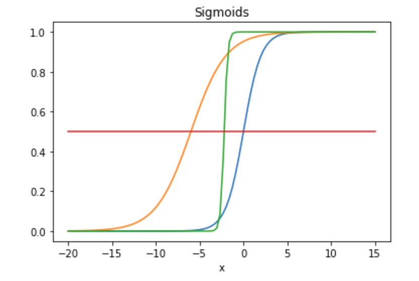
On the same plot, plot the sigmoid function and the custom sigmoids defined as:

sigmoid1(x) = 1/(1+ exp(-(0.5*x + 3)))
sigmoid2(x) = 1/(1+ exp(-(5*x + 11)))
Add a line representing the probability=0.5

The plot should look like this:

Exercise 3: Decision boundary

The goal of this exercise is to learn to fit a logistic regression on simple examples and to understand how the algorithm separated the data from the different classes.

1 dimension

First, we will start as usual with features data in 1 dimension. Use make classification from Scikit-learn to generate 100 data points:

X,y = make_classification(
    n_samples=100,
    n_features=1,
    n_informative=1,
    n_redundant=0,
    n_repeated=0,
    n_classes=2,
    n_clusters_per_class=1,
    weights=[0.5,0.5],
    flip_y=0.15,
    class_sep=2.0,
    hypercube=True,
    shift=1.0,
    scale=1.0,
    shuffle=True,
    random_state=88
)

Warning: The shape of X is not the same as the shape of y. You may need (for some questions) to reshape X using: X.reshape(1,-1)[0].

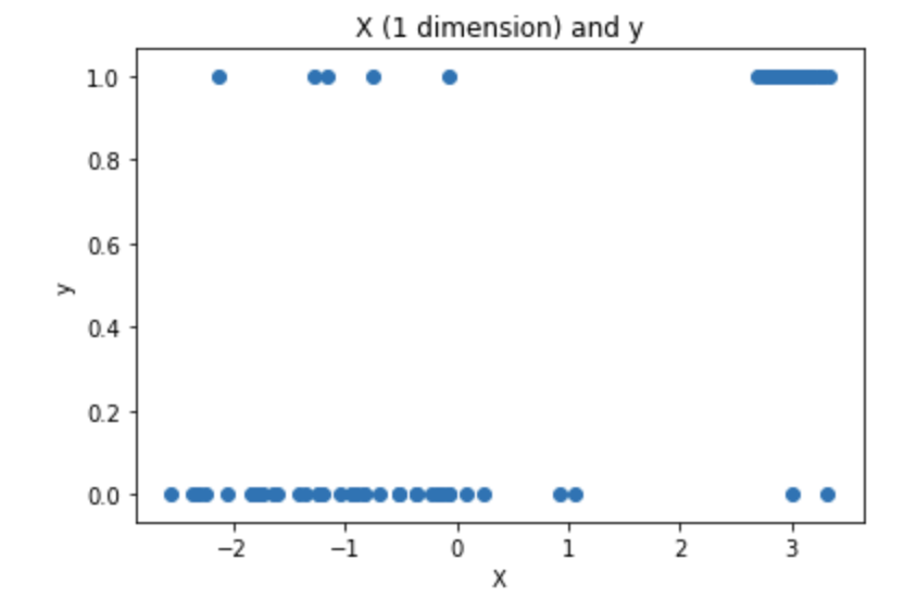
Plot the data using a scatter plot. The x-axis contains the feature and y-axis contains the target.

The plot should look like this:

Fit a Logistic Regression on the generated data using scikit learn. Print the coefficients and the interception of the Logistic Regression.
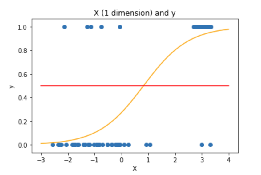
Add to the previous plot the fitted sigmoid and the 0.5 probability line. The plot should look like this:

Create a function predict_probability that takes as input the data point and the coefficients and that returns the predicted probability. As a reminder, the probability is given by: p(x) = 1/(1+ exp(-(coef*x + intercept))). Check you have the same results as the method predict_proba from Scikit-learn.

def predict_probability(coefs, X):
    '''
    coefs is a list that contains a and b: [coef, intercept]
    X is the features set

    Returns probability of X
    '''
    #TODO
    probabilities =

    return probabilities

Create a function predict_class that takes as input the data point and the coefficients and that returns the predicted class. Check you have the same results as the class method predict output on the same data.
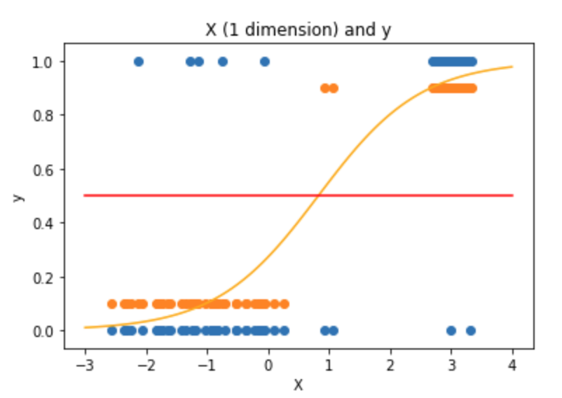
On the plot add the predicted class. The plot should look like this (the predicted class is shifted a bit to make the plot more understandable, but obviously the predicted class is 0 or 1, not 0.1 or 0.9) The plot should look like this:

2 dimensions

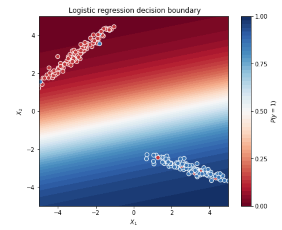
Now, let us repeat this process on 2-dimensional data. The goal is to focus on the decision boundary and to understand how the Logistic Regression create a line that separates the data. The code to plot the decision boundary is provided, however it is important to understand the way it works.

Generate 500 data points using:

X, y = make_classification(n_features=2,
                           n_redundant=0,
                           n_samples=250,
                           n_classes=2,
                           n_clusters_per_class=1,
                           flip_y=0.05,
                           class_sep=3,
                           random_state=43)

Fit the Logistic Regression on X and y and use the code below to plot the fitted sigmoid on the data set.

The plot should look like this:

xx, yy = np.mgrid[-5:5:.01, -5:5:.01]
grid = np.c_[xx.ravel(), yy.ravel()]
#if needed change the line below
probs = clf.predict_proba(grid)[:, 1].reshape(xx.shape)

f, ax = plt.subplots(figsize=(8, 6))
contour = ax.contourf(xx, yy, probs, 25, cmap="RdBu",
                      vmin=0, vmax=1)
ax_c = f.colorbar(contour)
ax_c.set_label("$P(y = 1)$")
ax_c.set_ticks([0, .25, .5, .75, 1])

ax.scatter(X[:,0], X[:, 1], c=y, s=50,
           cmap="RdBu", vmin=-.2, vmax=1.2,
           edgecolor="white", linewidth=1)

ax.set(aspect="equal",
       xlim=(-5, 5), ylim=(-5, 5),
       xlabel="$X_1$", ylabel="$X_2$")

The plot should look like this:

https://stackoverflow.com/questions/28256058/plotting-decision-boundary-of-logistic-regression

Exercise 4: Train test split

The goal of this exercise is to learn to split a classification data set. The idea is the same as splitting a regression data set but there's one important detail specific to the classification: the proportion of each class in the train set and test set.

   X = np.arange(1,21).reshape(10,-1)
   y = np.zeros(10)
   y[7:] = 1

Split the data using train_test_split with shuffle=False. The test set represents 20% of the total size of the data set. Print X_train, y_train, X_test, y_test. Compute the proportion of class 1 on the train set and test set.
Having a train set with different properties than the test set is not recommended. The analogy of the exam (https://www.youtube.com/watch?v=_vdMKioCXqQ) helps to understand this point: if the questions you have at the exam are completely different from what you prepared for you are not evaluated on what you learn. The training set has to be representative of the data set. Now, split the data in a train set and test set, but keep the proportion of class 1 nearly constant. The parameter shuffle in theory works as it relies on a random sampling. The parameter stratify will always split the data and keep the same proportion of class 1 in the train set and test set. Using the parameter stratify split the data below and print the proportion of class 1 in the train set and train set.

X = np.arange(1,201).reshape(100,-1)
y = np.zeros(100)
y[70:] = 1

Exercise 5: Breast Cancer prediction

The goal of this exercise is to use Logistic Regression to predict breast cancer. It is always important to understand the data before training any Machine Learning algorithm. The data is described in breast-cancer-wisconsin.names. I suggest to add manually the column names in the DataFrame.

Preliminary:

If needed, replace missing values with the median of the column.
Handle the column Sample code number. This column won't be used to train the model as it doesn't contain information on breast cancer. There are two solutions: drop it or set it as index.

Print the proportion of class Benign. What would be the accuracy if the model always predicts Benign? Later this week we will learn about other metrics as AUC that will help us to tackle high imbalanced data sets.
Using train_test_split, split the data set in a train set and test set (20%). Both sets should have approximately the same proportion of class Benign. Use random_state = 43.
Fit the logistic regression on the train set. Predict on the train set and test set. Compute the score on the train set and test set. 92-97% accuracy is expected on the test set.
Compute the confusion matrix on both tests. Analyse the number of false negative and false positive.

Exercise 6: Multi-class (Optional)

The goal of this exercise is to learn to train a classification algorithm on a multi-class labelled data. Some algorithms as SVM or Logistic Regression do not natively support multi-class (more than 2 classes). There are some approaches that allow to use these algorithms on multi-class data. Let's assume we work with 3 classes: A, B and C.

One-vs-Rest considers 3 binary classification problems: A vs B,C; B vs A,C and C vs A,B. If there are 10 classes, 10 binary classification problems would be fitted.
One-vs-One considers 3 binary classification problems: A vs B, A vs C, B vs C. If there are 10 classes, 45 binary classification problems would be fitted. Given, the volume of data, this technique may not be scalable.

More details:

https://machinelearningmastery.com/one-vs-rest-and-one-vs-one-for-multi-class-classification/

Let's implement the One-vs-Rest approach from LogisticRegression.

Preliminary:

Import the Setosa data set from Scikit-learn

from sklearn.datasets import load_iris
iris = load_iris()

X = pd.DataFrame(data=iris['data'], columns=iris.feature_names)
y = pd.DataFrame(data=iris['target'], columns=['target'])

Using train_test_split, split the data set in a train set and test set (20%) with shuffle=True and random_state=43.

Create a function that takes as input the data and returns three trained classifiers.

clf0 takes as input a binary data set where the class 1 is 0 and class 0 is 1 and 2.
clf1 takes as input a binary data set where the class 1 is 1 and class 0 is 0 and 2.
clf2 takes as input a binary data set where the class 1 is 2 and class 0 is 0 and 1.

def train(X_train,y_train):
       #TODO
       return clf0, clf1, clf2

Create a function that takes as input the trained classifiers and the features set and that returns the predicted class. Use predict_one_vs_all to output the predicted classes on the test set. Compare the results with Logistic Regression algorithm from scikit learn used in One-vs-All mode. The results may change because the solver may not converge. Later this week, we will learn to preprocess the data to avoid convergence issues.

clf0 outputs the probability to belong to the class 1 which is 0.
clf1 outputs the probability to belong to the class 1 which is 1.
clf2 outputs the probability to belong to the class 1 which is 2.

The predicted class is the one that gets the highest probability among the three models.

def predict_one_vs_all(X, clf0, clf1, clf2 ):
       #TODO
       return classes