public/subjects/ai/linear-regression/README.md

Linear regression

The goal of this day is to understand practical Linear regression and supervised learning with Scikit Learn.

The word "regression" was introduced by Sir Francis Galton (a cousin of C. Darwin) when he studied the size of individuals within a progeny. He was trying to understand why large individuals in a population appeared to have smaller children, more close to the average population size; hence the introduction of the term "regression".

Today we will learn a basic algorithm used in supervised learning : The Linear Regression. We will be using Scikit-learn which is a machine learning library. It is designed to interoperate with the Python libraries NumPy and Pandas.

We will also learn progressively the Machine Learning methodology for supervised learning - today we will focus on evaluating a machine learning model by splitting the data set in a train set and a test set.

Exercises of the day

• Exercise 0: Environment and libraries
• Exercise 1: Scikit-learn estimator
• Exercise 2: Linear regression in 1D
• Exercise 3: Train test split
• Exercise 4: Forecast diabetes progression
• Exercise 5: Gradient Descent (Optional)

Virtual Environment

• Python 3.x
• NumPy
• Pandas
• Matplotlib
• Scikit Learn
• Jupyter or JupyterLab

Version of Scikit Learn I used to do the exercises: 0.22. I suggest using the most recent one. Scikit Learn 1.0 is finally available after ... 14 years.

Resources

To start with Scikit-learn

• https://scikit-learn.org/stable/tutorial/basic/tutorial.html

• https://jakevdp.github.io/PythonDataScienceHandbook/05.02-introducing-scikit-learn.html

• https://scikit-learn.org/stable/modules/linear_model.html

Machine learning methodology and algorithms

• This course provides a broad introduction to machine learning, data mining, and statistical pattern recognition. Andrew Ng is a star in the Machine Learning community. I recommend spending some time during the projects to focus on some algorithms. However, Python is not the language used for the course. https://www.coursera.org/learn/machine-learning

• https://docs.microsoft.com/en-us/azure/machine-learning/algorithm-cheat-sheet

• https://scikit-learn.org/stable/tutorial/index.html

Linear Regression

• https://towardsdatascience.com/laymans-introduction-to-linear-regression-8b334a3dab09

• https://towardsdatascience.com/linear-regression-the-actually-complete-introduction-67152323fcf2

Train test split

• https://machinelearningmastery.com/train-test-split-for-evaluating-machine-learning-algorithms/

• https://developers.google.com/machine-learning/crash-course/training-and-test-sets/video-lecture?hl=en

---

---

Exercise 0: Environment and libraries

The goal of this exercise is to set up the Python work environment with the required libraries.

Note: For each quest, your first excerise will be to set up the virtual environment with the required libraries.

I recommend to use:

• the last stable versions of Python.
• the virtual environment you're the most comfortable with. virtualenv and conda are the most used in Data Science.
• one of the most recent versions of the libraries required

1. Create a virtual environment named ex00, with a version of Python >= 3.8, with the following libraries: pandas, numpy, jupyter, matplotlib and scikit-learn.

---

---

Exercise 1: Scikit-learn estimator

The goal of this exercise is to learn to fit a Scikit-learn estimator and use it to predict.

X, y = [[1],[2.1],[3]], [[1],[2],[3]]

1. Fit a LinearRegression from Scikit-learn with X the features and y the target and predict for x_pred = [[4]]

2. Print the coefficients (coefs_) and the intercept (intercept_), the score (score) of the regression of X and y.

---

---

Exercise 2: Linear regression in 1D

The goal of this exercise is to understand how the linear regression works in one dimension. To do so, we will generate a data in one dimension. Using make regression from Scikit-learn, generate a data set with 100 observations:

X, y, coef = make_regression(n_samples=100,
                         n_features=1,
                         n_informative=1,
                         noise=10,
                         coef=True,
                         random_state=0,
                         bias=100.0)

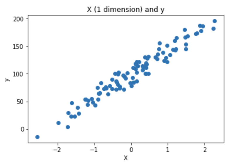
1. Plot the data using matplotlib. The plot should look like this:

2. Fit a LinearRegression from Scikit-learn on the generated data and give the equation of the fitted line. The expected output is: y = coef * x + intercept

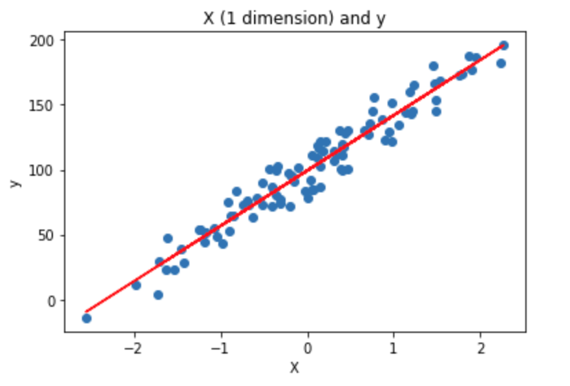
3. Add the fitted line to the plot. The plot should look like this:

4. Predict on X.

5. Create a function that computes the Mean Squared Error (MSE) and compute the MSE on the data set. The MSE is frequently used as well as other regression metrics that will be studied later this week.

   def compute_mse(y_true, y_pred):
       #TODO
       return mse
   

   Change the noise parameter of make_regression to 50

6. Repeat question 2, 4 and compute the MSE on the new data.

https://scikit-learn.org/stable/modules/generated/sklearn.metrics.mean_squared_error.html

---

---

Exercise 3: Train test split

The goal of this exercise is to learn to split a data set. It is important to understand why we split the data in two sets. To put it in a nutshell: the Machine Learning model learns on the training data and evaluates on the data the model hasn't seen before: the testing data.

This video gives a basic and nice explanation: https://www.youtube.com/watch?v=_vdMKioCXqQ

This article explains the conditions to split the data and how to split it: https://machinelearningmastery.com/train-test-split-for-evaluating-machine-learning-algorithms/

X = np.arange(1,21).reshape(10,-1)
y = np.arange(1,11)

1. Split the data using train_test_split with shuffle=False. The test set represents 20% of the total size of the data set. Print X_train, y_train, X_test, y_test.

https://scikit-learn.org/stable/modules/generated/sklearn.model_selection.train_test_split.html

---

---

Exercise 4: Forecast diabetes progression

The goal of this exercise is to use Linear Regression to forecast the progression of diabetes. It will not always be precised, you should ALWAYS start doing an exploratory data analysis in order to have a good understanding of the data you model. As a reminder here an introduction to EDA:

• https://towardsdatascience.com/exploratory-data-analysis-eda-a-practical-guide-and-template-for-structured-data-abfbf3ee3bd9

The data set used is described in https://scikit-learn.org/stable/modules/generated/sklearn.datasets.load_diabetes.

from sklearn.datasets import load_diabetes
diabetes = load_diabetes(as_frame=True)
X, y = diabetes.data, diabetes.target

1. Using train_test_split, split the data set in a train set, and test set (20%). Use random_state=43 for results reproducibility.

2. Fit the Linear Regression on all the variables. Give the coefficients and the intercept of the Linear Regression. What is the equation ?

3. Predict on the test set. Predicting on the test set is like having new patients for who, as a physician, need to forecast the disease progression in one year given the 10 baseline variables.

4. Compute the MSE on the train set and test set. Later this week we will learn about the R2 which will help us to evaluate the performance of this fitted Linear Regression. The MSE returns an arbitrary value depending on the range of error.

WARNING: This will be explained later this week. But here, we are doing something "dangerous". As you may have read in the data documentation the data is scaled using the whole dataset whereas we should first scale the data on the training set and then use this scaling on the test set. This is a toy example, so let's ignore this detail for now.

https://scikit-learn.org/stable/datasets/toy_dataset.html#diabetes-dataset

---

---

Exercise 5: Gradient Descent (Optional)

The goal of this exercise is to understand how the Linear Regression algorithm finds the optimal coefficients.

The goal is to fit a Linear Regression on a one dimensional features data without using Scikit-learn. Let's use the data set we generated for the exercise 2:

X, y, coef = make_regression(n_samples=100,
                         n_features=1,
                         n_informative=1,
                         noise=10,
                         coef=True,
                         random_state=0,
                         bias=100.0)

Warning: The shape of X is not the same as the shape of y. You may need (for some questions) to reshape X using: X.reshape(1,-1)[0].

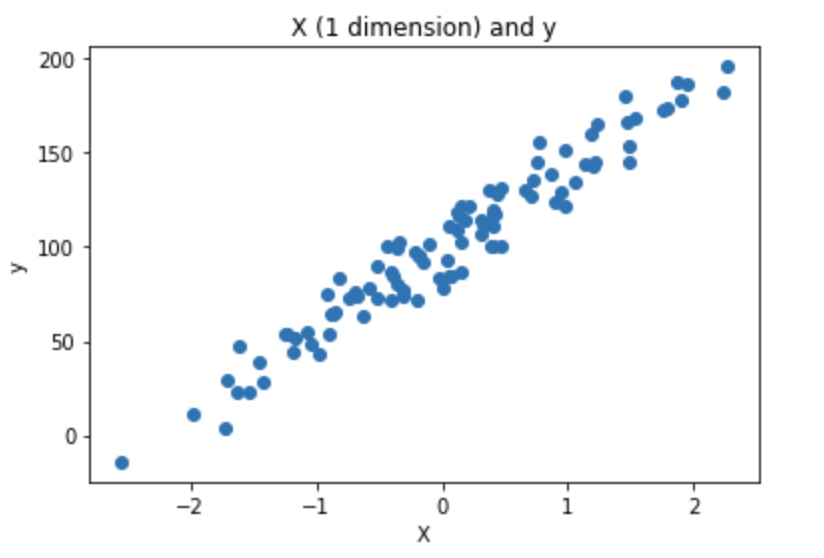
1. Plot the data using matplotlib:

As a reminder, fitting a Linear Regression on this data means finding (a, b) that fits well the data points.

• y_pred = a*x +b

Mathematically, it means finding (a, b) that minimizes the MSE, which is the loss used in Linear Regression. If we consider 3 data points:

• Loss(a,b) = MSE(a,b) = 1/3 *((y_pred1 - y_true1)**2 + (y_pred2 - y_true2)**2) + (y_pred3 - y_true3)**2)

and we know:

y_pred1 = ax1 + b
y_pred2 = ax2 + b
y_pred3 = a*x3 + b

Greedy approach

2. Create a function compute_mse. Compute mse for a = 1 and b = 2. Warning: X.shape is (100, 1) and y.shape is (100, ). Make sure that y_preds and y have the same shape before to compute y_preds-y.

def compute_mse(coefs, X, y):
    '''
    coefs is a list that contains a and b: [a,b]
    X is the features set
    y is the target

    Returns a float which is the MSE
    '''

    #TODO

    y_preds =
    mse =

    return mse

3. Create a grid of 640000 points that combines a and b with. Check that the grid contains 640000 points.

• a between -200 and 200, step= 0.5
• b between -200 and 200, step= 0.5

This is how to compute the grid with the combination of a and b:

aa, bb = np.mgrid[-200:200:0.5, -200:200:0.5]
grid = np.c_[aa.ravel(), bb.ravel()]

4. Compute the MSE for all points in the grid. If possible, parallelize the computations. It may be needed to use functools.partial to parallelize a function with many parameters on a list. Put the result in a variable named losses.

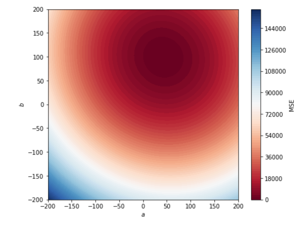
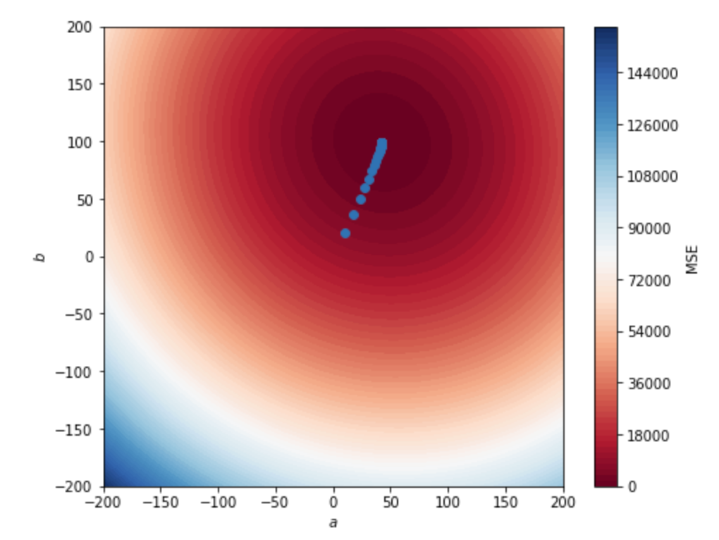
5. Use this chunk of code to plot the MSE in 2D:

aa, bb = np.mgrid[-200:200:.5, -200:200:.5]
grid = np.c_[aa.ravel(), bb.ravel()]
losses_reshaped = np.array(losses).reshape(aa.shape)

f, ax = plt.subplots(figsize=(8, 6))
contour = ax.contourf(aa,
                    bb,
                    losses_reshaped,
                    100,
                    cmap="RdBu",
                    vmin=0,
                    vmax=160000)
ax_c = f.colorbar(contour)
ax_c.set_label("MSE")

ax.set(aspect="equal",
    xlim=(-200, 200),
    ylim=(-200, 200),
    xlabel="$a$",
    ylabel="$b$")

The expected output is:

6. From the losses list, find the optimal value of a and b and plot the line in the scatter point of question 1.

In this example we computed 160 000 times the MSE. It is frequent to deal with 50 features, which requires 51 parameters to fit the Linear Regression. If we try this approach with 50 features we would need to compute 5.07e+132 MSE. Even if we reduce the scope and try only 5 values per coefficients we would have to compute the MSE 4.4409e+35 times. This approach is not scalable and that is why is not used to find optimal coefficients for Linear Regression.

Gradient Descent

In a nutshell, Gradient descent is an optimization algorithm used to minimize some function by iteratively moving in the direction of steepest descent as defined by the negative of the gradient. In machine learning, we use gradient descent to update the parameters (a and b) of our model. Parameters refer to the coefficients used in Linear Regression. Before to start implementing the questions, take the time to read this article. It explains the gradient descent and how to implement it. The "tricky" part is the computation of the derivative of the mse. You can admit the formulas of the derivatives to implement the gradient descent (d_theta_0 and d_theta_1 in the article).

7. Implement the gradient descent to find optimal a and b with learning rate = 0.1 and nbr_iterations=100.

8. Save the a and b through the iterations in a two-dimensional numpy array. Add them to the plot of the previous part and observe a and b that converge towards the minimum. The plot should look like this:

9. Use Linear Regression from Scikit-learn. Compare the results.